6. Spatial Network analysis¶

Task 1: Warmup poll! What kind of networks surround us?

Name a network of any kind that comes to your mind, which is somehow relevant for your own life? Add your suggestion here (click the link).

Introduction¶

Networks are everywhere. Social networks, telecommunication networks, neural networks, and transportation networks are all familiar examples how the networks surround us and are very essential to our everyday life. No surprise then, that studying complex networks has grown to be a very important topic in various fields of science including biology, medical sciences, social science, engineering, geography and many others.

Examples of different kind of networks:

Lesson objectives¶

Today we will focus on spatial networks and learn different methods for analyzing spatial networks and conduct useful queries such as finding the shortest path along a street network.

Learning goals

After this tutorial, you should be able to:

Understand typical application areas for spatial network analysis
Know the basic concepts and elements of a graph (network)
Be able to solve simple spatial network analysis problems using Python programming language

Additional materials

Literature

De Smith, Goodchild, Longley et al. (2020). Geospatial Analysis - Chapter 7: Network and Location Analysis

Videos

Exercise 6

In Exercise 6, you will practice how to work with OpenStreetMap data and conduct network analysis in Python. The practical programming sessions will be organized again on Thursday where you can get help from the course assistants.

You can start working on your copy of Exercise 6 by accepting the GitHub Classroom assignment.

Before we dive deeper to spatial networks, let’s spend a moment with the following task:

Task 2: Post your ideas to the chat!

Can you think of any practical examples where spatial network analysis algorithms are used in daily operations of the society?

1. Navigation

Show me the best route from A to B:

Car navigation
Journey planning (public transport)
Emergency way-finding etc.

Source: Sygic Ltd (2020)¶

2. Spatial planning

Where should we locate a new service?
Where traffic congestion is most likely going to worsen in the future? (simulations)
How many people can reach this location within X minutes?

How fast do you reach different parts of the city by different travel modes? (pink: private car, yellow: bicycle, green: public transport) Source: Topi Tjukanov (2018)¶

3. Spatial economics

Forecasting economic developments in the area
How many more customers/revenue this shop is going to get when the new metro-line opens?
Spatial interaction models (e.g. gravity models such as Huff’s)

Source Ela Dramowicz (2015)¶

Tutorial¶

In this tutorial we will focus on a network analysis methods that relate to way-finding. Finding a shortest path from A to B using a specific street network is a very common spatial analytics problem that has many practical applications.

Python provides easy to use tools for conducting spatial network analysis. One of the easiest ways to start is to use a library called Networkx which is a Python module that provides a lot tools that can be used to analyze networks on various different ways. It also contains algorithms such as Dijkstra’s algorithm or A* algoritm that are commonly used to find shortest paths along transportation network.

Next, we will learn how to do spatial network analysis in practice.

What is a graph?¶

Before continuing, it is good to understand some basic things about a graph that is the underlying data structure used when conducting routing.

Graphs are, in principle, very simple data structures, and they consists of:

nodes (e.g. intersections on a street, or a person in social network), and
edges (a link that connects the nodes to each other)

A simple graph could look like this:

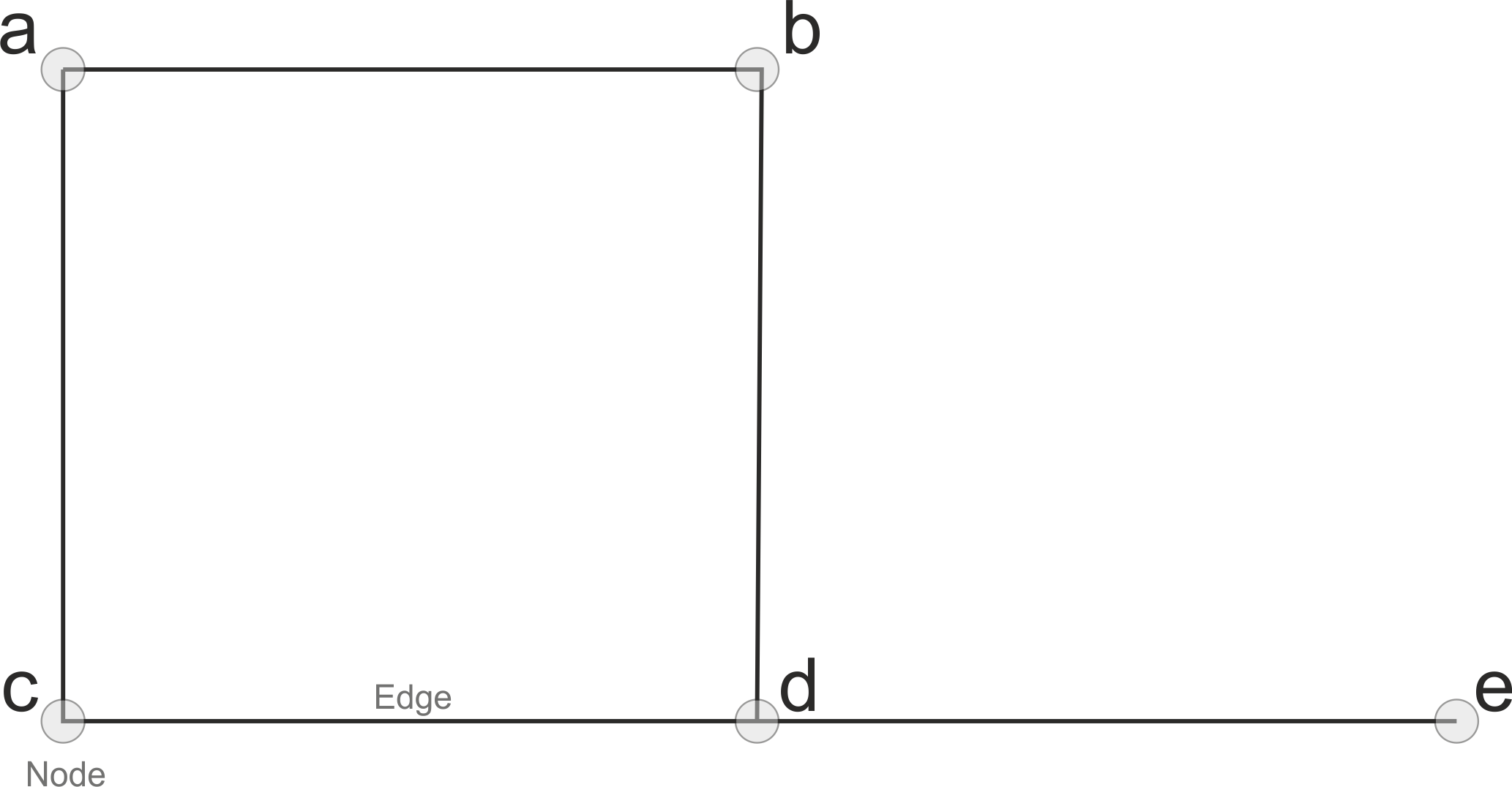
A simple graph.¶

Here, the letters A, B, C, D, and E are nodes and the lines that goes between them are edges/links.

Node and Edge attributes¶

In terms of street networks, nodes typically contain the geographical information associated with the graph (i.e. coordinates of the intersection). Edges typically contain much more information. They e.g. contain information about which nodes are connected to each other, and what is the cost to travel between the nodes (e.g. time, distance, CO2, etc.). It is also possible to associate geographical information to edges (if you e.g. want to show how the roads are curved between intersections), but for basic travel time analyses this is not needed.

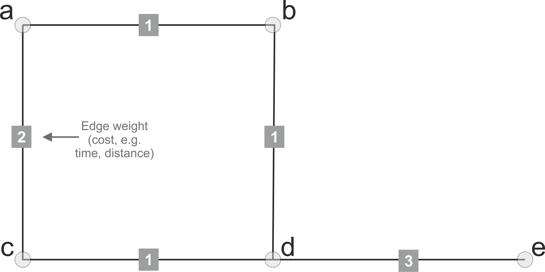
Graph with weights.¶

Directed vs Undirected graphs¶

Graph can be directed or undirected, which basically determines whether the roads can be travelled to any direction or whether the travel direction is restricted to certain direction (e.g. a one-way-street).

In undirected graph, it is possible to travel in both directions between nodes (e.g. from A --> C and from C --> A). Undirected graphs are typically used e.g. with walking and cycling as with those travel modes it is typically possible to travel the same street in any direction you like.

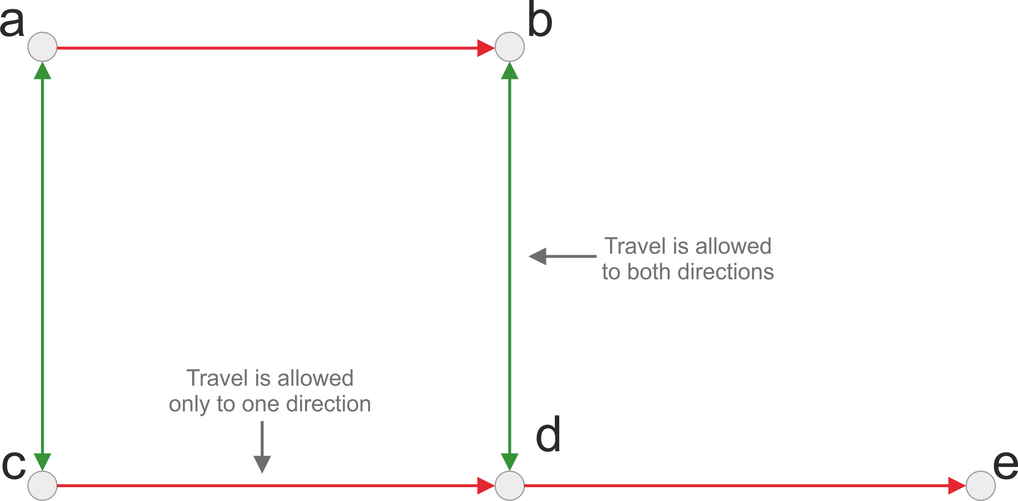
Directed graph.¶

If the graph is directed, it means that you should have a separate edge for each direction. If you for example have a graph with only an edge that goes from D to E, you can travel to node E from D but you cannot travel back. In directed graphs, you need to have a separate edge for each travel direction. Fundamentally this means that for a bi-directional road, you should have edges in your data (i.e. two separate rows), such as:

edge_id	from_node	to_node	description
1	A	C	edge for direction 1
2	C	A	edge for direction 2

TASK 3 - Vote!

The following routes are examples of paths with costs along the network. Which one is faster? Choose A or B. (press + to open the quiz)

Questions (open in full screen if difficult to see)

Next, we will continue, and see how to conduct shortest path analysis by walking/cycling using Python.

Typical workflow for spatial network analysis¶

If you want to conduct network analysis (in any programming language) there are a few basic steps that needs to be done before you can start routing (remember the workflow that we learned during the first lesson).

These steps are:

Retrieve data (such as street network from OSM or Digiroad + possibly transit data if routing with PT).
(Possibly modify the network by applying custom edge weights considering e.g. traffic conditions for car).
Build a routable graph for the routing tool that you are using (e.g. NetworkX, Igraph or OpenTripPlanner).
Conduct network analysis (such as shortest path analysis) with the routing tool of your choice.
Visualize the results (e.g. the shortest paths on the map, or isochrones)

Network analysis by walking / cycling¶

1. Retrieve data¶

As a first step, we need to obtain data for routing. OSMnx library makes it really easy to retrieve routable networks from OpenStreetMap with different transport modes (walking, cycling and driving). Osmnx also combines some functionalities from networkx module to make it straightforward to conduct routing along OpenStreetMap data.

Let’s first download the OSM data from Kamppi that are walkable. In OSMnx, we can use a function called .graph_from_place() which retrieves data from OpenStreetMap. It is possible to specify what kind of roads should be retrieved from OSM with network_type -parameter.

Okay, so as we can see the OSMnx library fetched some data and returned us a MultiDiGraph object.

Let’s see what the data looks like:

As we can see, now we have fetched walkable streets from Kamppi. In the figure, the lines are streets and all the nodes are represented with light blue color.

How does the actual data look like?

There are a couple of ways to access the edge and node attributes. The easier way is to use an OSMnx function graph_to_gdfs() that returns the nodes and edges as GeoDataFrames. The other option to access the data is via the graph itself by looping through nodes and edges as follow: - for node_id, node in G.nodes(data=True) - for fr, to, edge in G.edges(data=True)

Often you want to manipulate nodes and edges somehow. Hence, often it is useful to fetch the data into GeoDataFrames:

As we can see from this edge-table, we have a lot of information. For routing purposes, the most useful attributes are length (in meters) and maxspeed (for car routing) which we can use to calculate travel times.

2. Modify the graph¶

Let’s next modify the data in our graph, so that we can conduct the shortest path search based on travel time.

In this case, we specify that the walking speed is a static 4.5 kmph and cycling speed is 19 kmph. We will calculate the cost of travel (time) for each road segment (i.e. edge) into a new column walk_t that we can later use as a weight variable in routing (also known as impedance or cost).

3. Build graph¶

Now as we have calculated the travel time for our edges. We still need to convert our nodes and edges back to a NetworkX graph, so that we can start using it for routing. When using OSM data fetched with OSMnx this can be done easily with function ox.gdfs_to_graph(). Notice that this only works when using OSMnx library, we will later see in detail how the graphs are built from scratch which enables you to customize them.

Let’s build the graph with OSMnx:

Okay, now we have converted our data back into a NetworkX graph. Let’s ensure that our new edge attribute really exists:

Great, as we can see now we have a new edge attribute in our graph that we can use for routing.

4. Routing with NetworkX¶

Now we have everything we need to start routing with NetworkX (by walking and cycling). But first, let’s again go through some basics about routing.

Basic logic in routing¶

Most (if not all) routing algorithms work more or less in a similar manner. The basic steps for finding an optimal route from A to B, is to: 1. Find the nearest node for origin location * (+ get info about its node-id and distance between origin and node) 2. Find the nearest node for destination location * (+ get info about its node-id and distance between origin and node) 3. Use a routing algorithm to find the shortest path between A and B 4. Retrieve edge attributes for the given route(s) and summarize them (can be distance, time, CO2, or whatever)

* in more advanced implementations you might search for the closest edge

This same logic should be applied always when searching for an optimal route between a single origin to a single destination, or when calculating one-to-many -type of routing queries (producing e.g. travel time matrices).

Find the optimal route between two locations¶

Next, we will learn how to find the shortest path between two locations using Dijkstra’s algorithm.

First, let’s find the closest nodes for two locations that are located in the area. OSMnx provides a handly function for geocoding an address ox.geocode(). We can use that to retrieve the x and y coordinates of our origin and destination.

Okay, now we have coordinates for our origin and destination.

Find the nearest nodes¶

Next, we need to find the closest nodes from the graph for both of our locations. For calculating the closest point we use here 'haversine' formula to get the distance in meters (with return_dist=True).

Now we are ready to start the actual routing with NetworkX.

Find the fastest route by walking / cycling¶

Now we can do the routing and find the shortest path between the origin and target locations by using the dijkstra_path() function of NetworkX. For getting only the cumulative cost of the trip, we can directly use a function dijkstra_path_length() that returns the travel time without the actual path.

With weight -parameter we can specify the attribute that we want to use as cost/impedance. We have now three possible weight attributes available: 'length', 'walk_t' and 'bike_t'.

Let’s first calculate the routes between locations by walking and cycling, and also retrieve the travel times

Okay, that was it! Let’s now see what we got as results by visualizing the results.

5. Visualize the results¶

For visualization purposes, we can use a handy function again from OSMnx called ox.plot_graph_route() (for static) or ox.plot_route_folium() (for interactive plot).

Let’s first make static maps

Great! Now we have successfully found the optimal route between our origin and destination and we also have estimates about the travel time that it takes to travel between the locations by walking and cycling. As we can see, the route for both travel modes is exactly the same which is natural, as the only thing that changed here was the constant travel speed.

Let’s still finally see an example how you can plot a nice interactive map out of our results with OSMnx:

Calculate travel times from one to many locations¶

When trying to understand the accessibility of a specific location, you typically want to look at travel times between multiple locations (one-to-many) or use isochrones (travel time contours).

Let’s see how we can calculate travel times from the origin node, to all other nodes in our graph using NetworkX function single_source_dijkstra_path_length():

# What did we get?
walk_times

{298372995: 0,
 310042886: 4.3,
 298372997: 4.8,
 1377211668: 9.1,
 298372992: 10.1,
 298372994: 10.5,
 298372999: 14.6,
 298373001: 15.0,
 298275980: 20.4,
 1008235033: 58.6,
 298275990: 61.6,
 298275993: 63.1,
...
}

As we can see, the result is a dictionary where we have the node_id as keys and the travel time as values.

For visualizing this information, we need to join this data with the nodes. For doing this, we can first convert the result to DataFrame and then we can easily merge the information with the nodes GeoDataFrame.

Great! Now we have the travel times from origin to all other nodes in the graph.

Let’s finally merge the data with the nodes GeoDataFrame and visualize the results

As we can see, the node_id in the nodes GeoDataFrame can be found from the index of the gdf as well as from the column osmid.

Let’s merge these two datasets:

Okay, now we have also the travel times associated for each node.

Let’s visualize this:

Okay, as we can see now we have quickly calculated the travel times for each node in the graph using a single call.

If you would have for example a predefined grid, you could find the nearest node for each grid centroid to produce a more matrix-like result.

Alternative approach - Ego graph¶

Alternatively, it is possible to directly set a specific time limit and restrict how long the graph is travelled from the origin, and return that subgraph for the user.

Let’s see an example:

As we can see, with this approach we can retrieve a partial graph that we could for example visualize with different colors, or e.g. subset the extent of our accessibility analysis to cover only specific range from the source.